[스타터스 TIL] 53일차.SQL 실전 트레이닝 (9)

웅진X유데미 STARTERS/TIL (Today I Learned)

[스타터스 TIL] 53일차.SQL 실전 트레이닝 (9) - 미니 프로젝트 2

라밍쏭 2023. 4. 22. 16:52

728x90

1. 분석할 항목

✅ RFM을 통한 고객 유지

① 이탈률 → 앱 푸쉬 알림, 00님을위한 추천목록, ~~까지 사용할 수 있는 쿠폰 발급
② R이 3인값(휴면X) 안에서 F+M 을통해 1등급 부터 5등급까지 나눠 해택주기
③ 지역별 매출액 비교 : 지역별 top 3의 top3 도시

✅ 전체적인 고객 유지

④ 시간대 별 주문건수 변화 (00시부터 24시까지 6시간씩)

⑤ 계절성 확인(어느 분기 or 월에 전체적으로 소비가 늘어나는지) → 많이들 찾는 제품으로 중/하위 고객

⑥ 등급별 상위 판매 카테고리

2. 쿼리 작성

2.1 필요 컬럼만 있는 join table 생성

미리 필요한 테이블과 컬럼들을 선정하여 각 테이블을 조인한 테이블을 생성함

customers	orders	order_payments	products	reviews	order_items
customer_id	order_id	payment_sequential	product_id	review_id	order_item_id
customer_unique_id	order_status	payment_installments	product_category_name	review_score	price
customer_city	order_purchase_timestamp	payment_value		review_creation_date	freight_value
customer_state	order_delivered_customer_date

create table final_table1 as
select distinct c.customer_id, c.customer_unique_id , c.customer_state , c.customer_city
		, o.order_id, o.order_status , o.order_purchase_timestamp , o.order_delivered_customer_date 
		, oi.order_item_id , oi.price , oi.freight_value , r.review_id , r.review_score 
		, r.review_creation_date , p.product_id , p.product_category_name , op.payment_sequential 
		, op.payment_installments , op.payment_value 
from customers c  
left join orders o
	on o.customer_id  = c.customer_id  
left join reviews r 
	on r.order_id = o.order_id 
left join order_payments op 
	on op.order_id = o.order_id 
left join order_items oi 
	on oi.order_id =o.order_id 
left join products p 
	on p.product_id = oi.product_id;

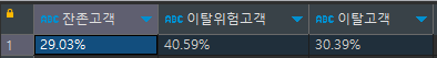
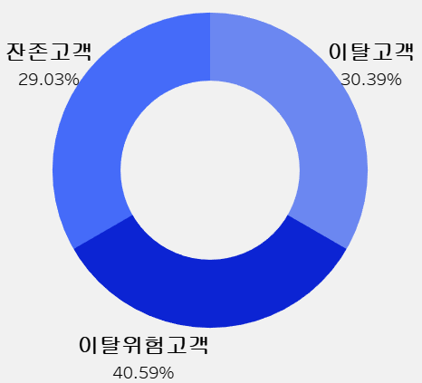
2.2 이탈률

- 우리가 설정한 RFM 지표를 기준으로 고객의 이탈률을 확인함

- 잔존고객의 비율이 작으며, 이탈위험고객과 이탈고객의 비율이 70%에 달하기 때문에

해당 고객들을 타겟으로 전략을 세우는 것이 신규고객을 타겟으로 하는 것보다 더 낫다고 판단함

✔ Recency가 3인 고객 : 잔존고객 → 29.03%

✔ Recency가 2인 고객 : 이탈위험고객 → 40.59%

✔ Recency가 1인 고객 : 이탈고객 → 30.39%

WITH 
cte_customers AS( --1. 필요 컬럼 추출 
SELECT DISTINCT customer_unique_id
		 , order_id
		 , date(order_purchase_timestamp) AS order_date
		 , payment_value AS sales
		 , max(date(order_purchase_timestamp)) over() AS std
		 , max(date(order_purchase_timestamp)) over() - date(order_purchase_timestamp) AS date_diff
FROM olist.final_table
) ,cte_rfm AS( --2. 고객 RFM 집계 
SELECT customer_unique_id
		 , COALESCE(min(date_diff), 0) AS recency
		 , COALESCE(count(DISTINCT order_id), 0) AS frequency
		 , COALESCE(sum(sales), 0) AS monetary
FROM cte_customers
GROUP BY 1
ORDER BY 1
), cte_score AS( --3. 고객 RFM 등급생성 
SELECT *
	 , CASE WHEN recency <= 180 THEN 3
	 		WHEN recency <= 360 THEN 2
	 		ELSE 1
	 		END AS r_score
	 , CASE WHEN frequency = 1 THEN 1
	 		WHEN frequency = 2 THEN 2
		 	ELSE 3
			END AS f_score
	 , CASE when monetary <= 63 then 1
			when monetary <= 108 then 2
			when monetary <= 183 then 3
			when monetary <= 624 then 4
			else 5
			end as m_score
FROM cte_rfm
) --4. 이탈률 확인 
SELECT round(((SELECT count(DISTINCT customer_unique_id) FROM cte_score WHERE r_score = 3) / count(*)::NUMERIC * 100), 2)::varchar(10)||'%' AS "잔존고객"
	 , round(((SELECT count(DISTINCT customer_unique_id) FROM cte_score WHERE r_score = 2) / count(*)::NUMERIC * 100), 2)::varchar(10)||'%' AS "이탈위험고객"
	 , round(((SELECT count(DISTINCT customer_unique_id) FROM cte_score WHERE r_score = 1) / count(*)::NUMERIC * 100), 2)::varchar(10)||'%' AS "이탈고객"
FROM cte_score;

2.3 등급 별 고객 수 + 비율

설정한 등급 별로 고객 수와 비율을 확인함

→ VVIP와 VIP는 매우 적게 차지하며, FAMILY (이탈 위험 고객)이 약 40%로 가장 많이 차지하는 것을 확인할 수 있음

✅ 등급 기준

VVIP	R(Recency) = 3	F(Frequency)+M(Monetary) = 6
VIP	R(Recency) = 3	F(Frequency)+M(Monetary) = 5
GOLD	R(Recency) = 3	F(Frequency)+M(Monetary) = 4
SILVER	R(Recency) = 3	F(Frequency)+M(Monetary) = 3
BRONZE	R(Recency) = 3	F(Frequency)+M(Monetary) = 2
FAMILY	R(Recency) = 2	-
SLEEPING	R(Recency) = 1	-

WITH cte_customers AS (
	SELECT DISTINCT customer_unique_id
		 , order_id
		 , date(order_purchase_timestamp) AS order_date
		 , payment_value AS sales
		 , max(date(order_purchase_timestamp)) over() AS std
		 , max(date(order_purchase_timestamp)) over() - date(order_purchase_timestamp) AS date_diff
	FROM final_table) -- 104,128개
, cte_rfm AS (
	SELECT DISTINCT customer_unique_id
		 , COALESCE(min(date_diff), 0) AS recency
		 , COALESCE(count(DISTINCT order_id), 0) AS frequency
		 , COALESCE(sum(sales), 0) AS monetary
	FROM cte_customers
	GROUP BY 1
	ORDER BY 1) -- 100,245개
, cte_score AS (
	SELECT *
		 , CASE WHEN recency <= 180 THEN 3
		 		WHEN recency <= 365 THEN 2
		 		ELSE 1
		   END AS r_score
		 , CASE WHEN frequency = 1 THEN 1
		 		WHEN frequency = 2 THEN 2
		 		ELSE 3
		 	END AS f_score
		 , CASE when monetary <= 108 then 1
				when monetary <= 364 then 2
				else 3
			end as m_score
	FROM cte_rfm
	ORDER BY r_score DESC, f_score DESC , m_score DESC)
, cte_grade AS (
	SELECT *
		 , CASE WHEN r_score = 3 AND f_score + m_score = 6 THEN 'VVIP'
		 		WHEN r_score = 3 AND f_score + m_score = 5 THEN 'VIP'
		 		WHEN r_score = 3 AND f_score + m_score = 4 THEN 'GOLD'
		 		WHEN r_score = 3 AND f_score + m_score = 3 THEN 'SILVER'
		 		WHEN r_score = 3 AND f_score + m_score = 2 THEN 'BRONZE'
		 		WHEN r_score = 2 THEN 'FAMILY'
		 		WHEN r_score = 1 THEN 'SLEEPING'
		 	END AS grade
	FROM cte_score)
, cte_grade_cnt AS (
	SELECT grade
		 , count(DISTINCT customer_unique_id) AS cnt
	FROM cte_grade
	GROUP BY grade)
SELECT *
	 , round((cnt / sum(cnt) over())::NUMERIC, 3) AS percent
FROM cte_grade_cnt
ORDER BY cnt;

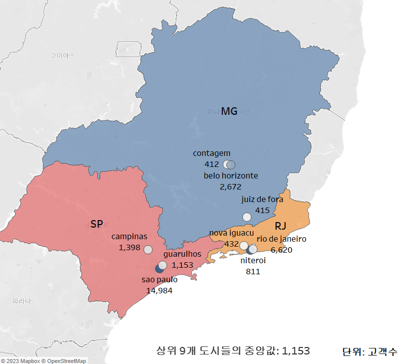
2.4 고객 수가 많은 지역의 도시 TOP 3

고객 수가 많은 지역 TOP3를 확인함

지역은 매우 넓기 때문에 마케팅 전략을 세우기 위해서는 좁은 범위의 도시를 확인하는 것이 더 낫다고 판단

→ 고객 수가 많은 TOP 3 지역 중에서 고객 수가 많은 도시 3개를 뽑음

✅ 등급을 추가한 최종 테이블 생성 (create table)

-- create table을 통해 grade가 붙은 최종 테이블 생성 
-- 1. 필요한 데이터 추출 
create table cte_select as
select distinct customer_unique_id, order_id, date(order_purchase_timestamp) as order_date , payment_value as sales 
     , max(date(order_purchase_timestamp)) over() as std_date
     , max(date(order_purchase_timestamp)) over() - date(order_purchase_timestamp) as date_diff
from final_table
;


-- 2. 고객별 RFM
create table cte_cust_rfm as
select customer_unique_id
     , coalesce (min(date_diff),0) as recency
     , coalesce (count(distinct order_id),0) as frequency
     , coalesce (sum(sales),0) as monetary
from cte_select 
group by 1
order by 1
;


--3. 점수부여 위한 구간 나누기 
create table olist.cte_cust_rfm_ntile as 
select customer_unique_id 
		, recency as r
		, case when recency <= 180 then 3
				when recency <= 365 then 2
				else 1 end as recency
		, frequency as f
		, case when frequency = 1 then 1 
				when frequency = 2 then 2
				else 3 end as frequency
		, monetary as m
		, case when monetary <= 108 then 1
		when monetary <= 364 then 2
		else 3 end as monetary
from olist.cte_cust_rfm
;


--4. 점수부여 위한 구간 나누기 
create table olist.cte_cust_rfm_score as 
select customer_unique_id ,recency,frequency, monetary, frequency+monetary as score 
		, case when recency=3 and frequency+monetary =2 then '5_grade'
			  when recency=3 and frequency+monetary =3 then '4_grade' 
			  when recency=3 and frequency+monetary =4 then '3_grade'	
			  when recency=3 and frequency+monetary =5 then '2_grade' 
			  when recency=3 and frequency+monetary =6 then '1_grade' 
			  when recency=2 then '등급없음'
			  else '휴면고객' end as grade 
from olist.cte_cust_rfm_ntile
;

--5. real_grade 추가 
create table olist.cte_cust_rfm_grade as 
select *
		, case when grade = '5_grade' then 'BRONZE'
				when grade = '4_grade' then 'SILVER' 
				when grade = '3_grade' then 'GOLD'	
				when grade = '2_grade' then 'VIP' 
				when grade = '1_grade' then 'VVIP' 
				when grade = '등급없음' then 'FAMILY'
				else 'SLEEPING' end as real_grade 
from olist.cte_cust_rfm_score
;

--6. 마지막 최종 테이블 생성 
create table olist.table_rfm as 
select ft.*, a.recency, a.frequency, a.monetary , a.score, a.grade, a.real_grade 
from olist.final_table ft
left join olist.cte_cust_rfm_grade a
	on ft.customer_unique_id = a.customer_unique_id
;

✅ 고객 수가 많은 지역의 도시 TOP 3

with cte_a as( --1. 필요 컬럼 추출 
select customer_unique_id, customer_state, customer_city 
from olist.table_rfm
group by 1,2,3
), cte_state as( --2.state별로 top3 city 
select customer_state, customer_city, count(distinct customer_unique_id)
		, row_number() over(partition by customer_state order by count(customer_unique_id) desc) as rank
from cte_a
where customer_state in ('SP', 'RJ', 'MG')
group by 1,2
order by 3,4 desc
), cte_pivot as( --3. rank로 pivot 
select customer_state
		, max(case when rank=1 then customer_city end) as rank_1
		, max(case when rank=2 then customer_city end) as rank_2
		, max(case when rank=3 then customer_city end) as rank_3
from cte_state
where rank <= 3 
group by 1
order by 1
)
select *
from cte_pivot
;

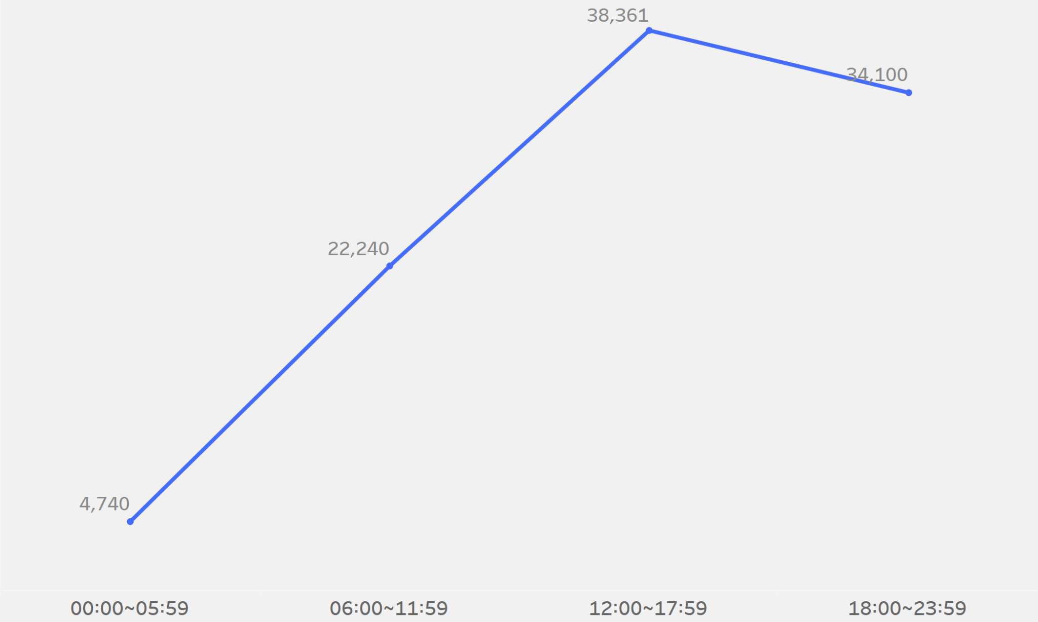
2.5 시간대 별 주문건수 변화

고객이 상품을 주문한 시간대 별로 주문건수를 확인하여 어느 시간대가 주문이 많은지를 확인하고자 함

→ 밤 12시 ~ 아침 6시가 가장 적으며, 오후 12시 ~ 오후 6시까지가 가장 많음

with
cte_table as( --1. 필요한 컬럼 추출 
select *
from final_table ft
), cte_time as( --2. 주문 시간대 grrup, 주문수 집계 
select extract(hour from order_purchase_timestamp) 시간
	, trunc(extract(hour from order_purchase_timestamp)/6) timesix
	, count(distinct order_id) 주문수
from cte_table
group by 1
order by 1
) --3. 시간대별 주문수 count 
select case 
	when timesix=0 then '00:00~05:59'
	when timesix=1 then '06:00~11:59'
	when timesix=2 then '12:00~17:59'
	when timesix=3 then '18:00~23:59'
	end as timesix_re
	, sum(주문수) otalnum
from cte_time
group by 1
order by 1
;

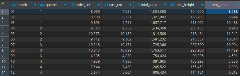
2.6 월 / 분기 별 주문건수 변화

분기별로 주문건수를 확인하고, 세부적으로 월 별로 주문건수를 확인하여 계절성을 파악하고자 함

→ 5월, 8월이 가장 주문건수가 많았으며, 9월에 주문건수가 급격히 줄어듦

→ 2분기가 가장 주문건수가 많았으며 4분기엔 주문건수가 줄어듦

with
cte_table as ( --1. 필요 컬럼만 추출 
select 	distinct to_char(order_purchase_timestamp, 'MM') as month
    	, to_char(order_purchase_timestamp, 'q') as quarter
    	, order_id, customer_unique_id, payment_value, freight_value 
from olist.table_rfm 
)  --2. 월, 분기별 주문건수, 고객수, 총 매출 확인 
select month, quarter
		, count(distinct order_id) as order_cnt
    	, count(distinct customer_unique_id) as cust_cnt
    	, round(sum(payment_value)) as total_sales
    	, round(sum(freight_value)) as total_freight
    	, count(*) as cnt_grade
from cte_table
group by 1,2
;

2.7 등급 별 TOP 5 판매 카테고리

등급 별로 가장 많이 주문을 한 카테고리를 순위로 나타냄

→ 각 등급 별로 해당하는 카테고리와 관련된 혜택 제공

with
cte_table as ( --1. 필요 컬럼만 추출 
select distinct product_category_name, real_grade, order_id
from olist.table_rfm 
), cte_rank as(--2. 등급별 각 카테고리 순위 확인 
select real_grade, product_category_name 
		, row_number() over(partition by real_grade order by count(product_category_name) desc) as rank
		, count(product_category_name) as count 
from cte_table
--where real_grade in ('FAMILY', 'SLEEPING')
group by 1,2
order by 1
),cte_pivot as( --3. rank기준으로 pivot 
select rank
		, max(case when real_grade='VVIP' then product_category_name end) as VVIP
		, max(case when real_grade='VIP' then product_category_name end) as VIP
		, max(case when real_grade='GOLD' then product_category_name end) as GOLD
		, max(case when real_grade='SILVER' then product_category_name end) as SILVER
		, max(case when real_grade='BRONZE' then product_category_name end) as BRONZE
		, max(case when real_grade='FAMILY' then product_category_name end) as FAMILY
		, max(case when real_grade='SLEEPING' then product_category_name end) as SLEEPING
from cte_rank
where rank <=10
group by 1
order by 1
), cte_avg as(--4. 모든 등급에서 카테고리의 평균 순위 
select product_category_name, round(avg(rank),1) as avg_rank 
	, rank() over(order by round(avg(rank),1)) as total_rank
from cte_rank
group by 1
order by 2
)
select * 
from cte_rank
where rank <=5;

3. 시각화

3.1 이탈률

3.2 등급 별 고객 수 + 비율

3.3 고객 수가 많은 지역의 도시 TOP 3

3.4 시간대 별 주문건수 변화

3.5 월 / 분기 별 주문건수 변화

3.6 등급별 TOP 5 판매 카테고리

4. 분석 진행 사항 (feat. Figma)

💡 회고

어제까지 진행한 분석 목적, 지표 설정, 분석 항목을 설정하였고 이를 바탕으로 하나씩 담당하여 쿼리를 짜고 결과값을 도출해내었다.

이 부분에서도 각자 짠 쿼리들을 서로 확인을 해보며 쿼리가 잘 짜여졌는지, 이렇게 결과값이 나오는 것이 맞는지를 확인하였다.

그리고 결과값을 바탕으로 시각화를 진행하였고, 결과값과 시각화를 한 것으로 발표자료를 만들었다.

(내일 TIL에 올릴 예정!)

다행히 제시간에 끝낼 수 있었으며, SQL 쿼리 연습이 많이 되어서 좋았다.

시간이 부족해서 주제를 선정할 때, 깊게 고민을 하지 않고 선정한 것이 조금 아쉽긴 하지만 그래도 결과물이 잘 나와서 만족스럽다! :)

728x90

'웅진X유데미 STARTERS > TIL (Today I Learned)' 카테고리의 다른 글

[유데미 스타터스 취업 부트캠프 4기] SQL 최종평가 공부 (쿼리) (0)	2023.04.22
[스타터스 TIL] 54일차.SQL 실전 트레이닝 (10) - 미니 프로젝트 3 (0)	2023.04.22
[스타터스 TIL] 52일차.SQL 실전 트레이닝 (8) - 미니프로젝트 1 (0)	2023.04.22
[스타터스 TIL] 51일차.SQL 실전 트레이닝 (7) - RFM 분석, 재구매율, 이탈고객 분석, 백분위수, 최빈값 (0)	2023.04.18
[스타터스 TIL] 50일차.SQL 실전 트레이닝 (6) - 고객 분석, Decil 분석, RFM 분석 (0)	2023.04.17

현재글[스타터스 TIL] 53일차.SQL 실전 트레이닝 (9) - 미니 프로젝트 2

ARAMDAUN

코딩테스트, SQL, Cos Pro 2급, 데이터드리븐, 데이터시각화, 유데미, 유데미부트캠프, COS PRO 파이썬, 파이썬, 유데미큐레이션, Python, 스타터스부트캠프, MySQL, 유데미코리아, 부트캠프후기, 데이터분석, 취업부트캠프, 파이썬 코딩테스트, 백준, 태블로,

Today :
Yesterday :

ARAMDAUN